68 Behavioral Parameters of Swiss Worker Schedule Flexibility

Maximum-likelihood estimation on 10,110 real microcensus schedules, the empirical calibration any activity-based travel-demand model can drop in instead of guessing

When two activities collide on someone's day, which one moves? Does a Swiss commuter stretch lunch or shorten work? Will they push leisure later, or skip it? Until now, transport models filled in those numbers by guesswork.

We worked with SBB and EPFL on the published journal paper that pulls them straight from data. The result is an empirical, peer-reviewed answer to how flexible each part of a Swiss working day really is, and the foundation for SBB's behavioral calibration of SIMBA MOBi.

68 / 68

behavioral parameters estimated from real data, every one significant at 5%

10,110

real Swiss microcensus schedules in the calibration sample

Transportation · Springer

peer-reviewed and open access (CC BY 4.0)

~1 hour

to simulate 50,000 Lausanne worker schedules on a 48-core server

The challenge

Existing activity-based models pick one flexibility coefficient per activity type, by hand. That can't capture that workers stretch lunch but rarely move their work block, or that shopping is more flexible than picking up a child.

SBB needed parameters grounded in observed Swiss behavior, estimated rigorously enough to defend a published model, and tractable enough to run in their full-population simulations.

Our approach

We treated flexibility as a vector of coefficients in a utility-maximizing MILP and estimated them by maximum likelihood against 10,110 cleaned schedules from the Swiss Mobility and Transport Microcensus, using the standard logit framework on a competitive choice set per individual.

We validated by running the estimated parameters back through the MILP for ≈ 50,000 full-time workers in Lausanne and comparing the simulated activity profiles against the empirical microcensus.

The outcome

Deliverable: a published, peer-reviewed empirical calibration of Swiss worker schedule flexibility, 68 statistically-significant behavioral parameters that any activity-based travel-demand model can drop in instead of guessing. The framework reaches ρ̄² = 0.154 against the 10,110-schedule sample and simulates ~45,000 Lausanne workers in roughly an hour on a 48-core server. Published open access in Transportation (Springer), CC BY 4.0.

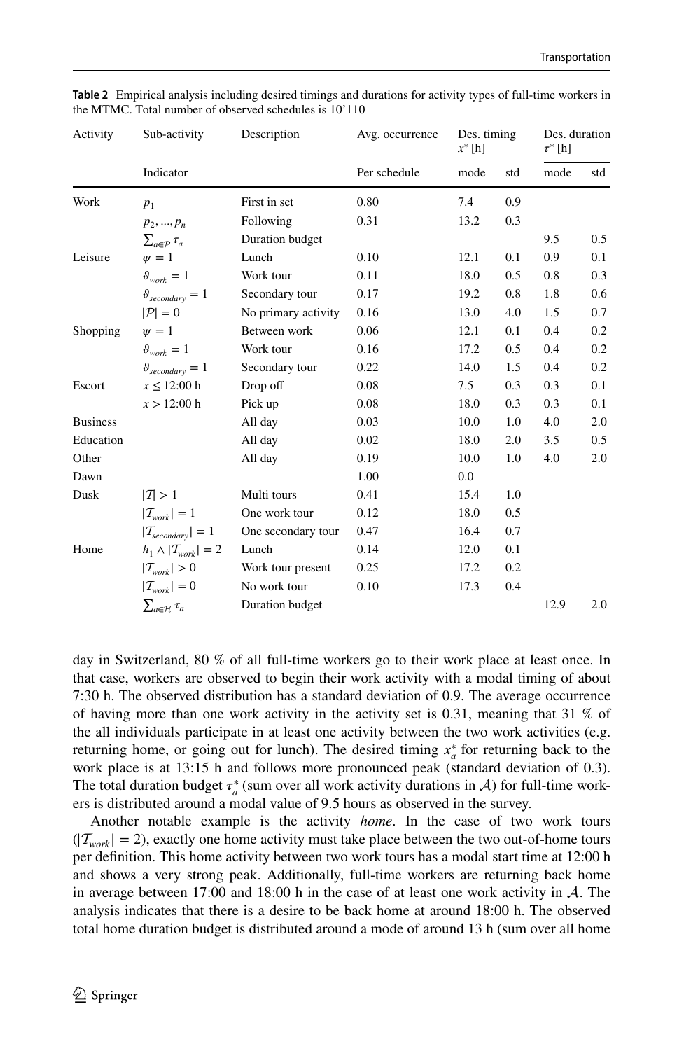
The behavioral picture is sharp: lunch is by far the most rigid activity in a Swiss worker's day (β^short = −7.61, roughly 350× more sensitive per hour to a short lunch than to a short workday). Morning work has a tight start-time target around 7:30, home-after-work pulls strongly toward 18:00, and evening leisure absorbs the residual flexibility. These are exactly the patterns travel-demand models need to calibrate against, but until now they were entered by hand instead of estimated from data.

Technical deep dive

The model behind the result.

The model

The total utility of a candidate schedule is decomposed into per-activity penalties for missing the desired start time and duration, plus a travel disutility on each leg. Each penalty is asymmetric: being early can hurt more or less than being late, and the same for duration.

U_{i} = a \in A_{i} \sum U_{timing} (x_{a}) + a \in S_{i} \sum U_{duration} (τ_{a}) + O \in {P_{i}, H_{i}} \sum U_{duration} (a \in O \sum τ_{a}) + a \in A_{i} ∖ {dusk} \sum β^{travel} t t_{a} .

Total schedule utility. Secondary activities are penalized individually; primary and home activities share a daily duration budget.

U_{timing} (x_{a}) = β_{a}^{early} max (0, x_{a}^{*} - x_{a}) + β_{a}^{late} max (0, x_{a} - x_{a}^{*}) .

Asymmetric piecewise-linear penalty around the desired start time x_a*. β^early and β^late are the parameters we estimate.

U_{duration} (τ_{a}) = β_{a}^{short} max (0, τ_{a}^{*} - τ_{a}) + β_{a}^{long} max (0, τ_{a} - τ_{a}^{*}) .

Mirror penalty around the desired duration τ_a*. β^short and β^long are estimated per activity cluster.

P_{n} (i ∣ C_{n}; β) = \frac{e ^{U_{i} (β)}}{\sum _{j \in C_{n}} e ^{U_{j} (β)}}, \hat{β} = ar g β max n = 1 \sum N lo g P_{n} (i_{n}^{*} ∣ C_{n}; β) .

Logit choice probability over the choice set C_n for individual n, and the maximum-likelihood objective over the realized schedule i*_n. Estimation runs in PandasBiogeme.

The estimator returns a single vector β̂ ∈ ℝ⁶⁸ that captures, in a single statistically defensible language, how rigid each cluster of activities is in a Swiss full-time worker's day.

Benchmark

Estimated flexibility preferences for selected activity clusters (Table 3 of the journal paper).

Activity / cluster	β^early	β^late	β^short	β^long
work : first in set	−0.518	−0.401	-	-
work : following	−0.317	0	-	-
work : daily duration budget	-	-	−0.022	0
leisure : lunch	−1.587	−0.760	−7.614	−1.314
leisure : evening secondary tour	−0.058	0	−3.087	−0.693
shopping : in a secondary tour	−0.229	−0.468	−6.003	−0.746
escort : drop off	−1.106	0	0	−4.171
home : lunch	−2.189	−1.067	-	-
home : with work tour present	−0.072	−0.397	-	-
home : daily duration budget	-	-	0	−0.373

Negative numbers are utility penalties per hour of deviation; 0 indicates the parameter was not significant at 5%. The strongest pattern: lunch is highly rigid (β^short = −7.61, workers really do not want a short lunch), and the home-at-lunch return is even stiffer than work itself. Morning work is twice as rigid as afternoon work in start time. Evening leisure absorbs flexibility. Sample size 10,110 cleaned full-time-worker schedules, 68 parameters all significant at 5%, ρ̄² = 0.154, log-likelihood improvement −57,443.43 → −48,548.23, estimation time ≈ 12.3 h on 40 cores.

From the record

Table 2 from the journal paper: empirical analysis of activity types in the Swiss microcensus. Each cluster is identified by a structural condition (e.g. 'sub-tour', 'between work', 'one secondary tour') and characterized by an average occurrence per schedule, a desired start time, and a desired duration with their standard deviations.

Figure 2 from the journal paper: simulated activity profiles for Lausanne full-time workers (left) versus the Swiss microcensus (right). The morning work peak, the 12:00 lunch dip, the evening leisure ramp and the home-overnight dominance are reproduced without any rule-based patching.

Figure 3 from the journal paper: 2D start-time × duration heatmaps for work and leisure activities, model versus microcensus. The bimodal work signature (long morning shift versus split-with-afternoon-return) and the lunch-leisure spike at 12:00 are recovered by the optimization alone.

Techniques

Maximum-likelihood estimation under a MILP simulator
Choice-set construction (likely + random alternatives)
Logit choice models on schedule alternatives
Continuous-time scheduling with piecewise-linear utility
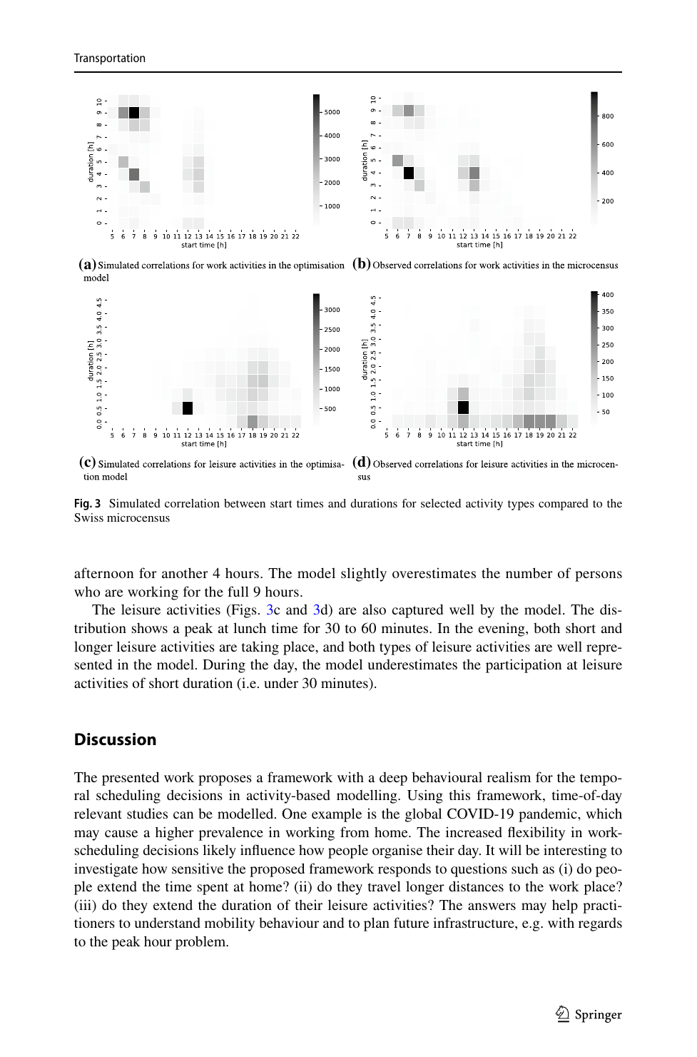
Validation via simulated activity profiles and 2D heatmaps

Stack

Python
PandasBiogeme
OR-Tools
SCIP
Ray (parallel execution)
Swiss MTMC microcensus

A problem like this?

We'd like to hear about it.

contact@optimally.ch