← Areas of expertise/Travel Demand · Estimation/2024

Joint Mode-and-Destination Choice Sets, Now Live in EPFL's OASIS Pipeline

First method to capture the mode/destination coupling jointly, with a closed-form bias-correction term that drops into any activity-based-model estimator

Activity-based travel models live or die on their choice sets. Use the universe of every possible destination and parameter estimation crawls. Use a naïve filter and you bias the model. Use rigid distance-based heuristics and you can't capture mode-destination interplay.

We co-authored a joint stochastic choice-set generation approach: estimate a cross-nested logit on observed mode-and-destination combinations, importance-sample from the resulting probability distribution, then perturb the sampled set with three random operators to inject unlikely alternatives, giving you realistic competitive sets for simulation and a controlled mix of likely/unlikely options for unbiased parameter estimation.

OASIS

now the choice-set-generation block of EPFL's ABM pipeline

Closed-form

bias-correction term drop-in for any ABM MLE estimator

Joint mode + destination

first method to capture the coupling, not just one axis at a time

STRC 2022

co-authored, validated on 3,536 Swiss microcensus trips

The challenge

Across decades of research, choice-set generation in activity-based modeling has been treated as a fixed, often arbitrary preprocessing step, typically based on rule-based distance or time filters (Hagerstrand's time-space prism, Schönfelder-Axhausen activity ellipses, Scherr et al.'s rubber-banding). The result is biased parameter estimates, degraded simulation realism, and no way to capture the genuine coupling between mode and destination decisions (a car gives you destinations you can't reach by public transport; needing to travel at peak hour makes closer destinations more attractive).

The challenge: build a method that generates choice sets which are simultaneously useful for simulation (competitive alternatives) and estimation (a controlled mix of likely and unlikely options), and that captures the interaction between mode and destination, not just one at a time. With 88 zones × 3 modes in even a small case study, that's 264 universal alternatives per individual; for Switzerland's 8,000 zones the universal set is 24,000.

Our approach

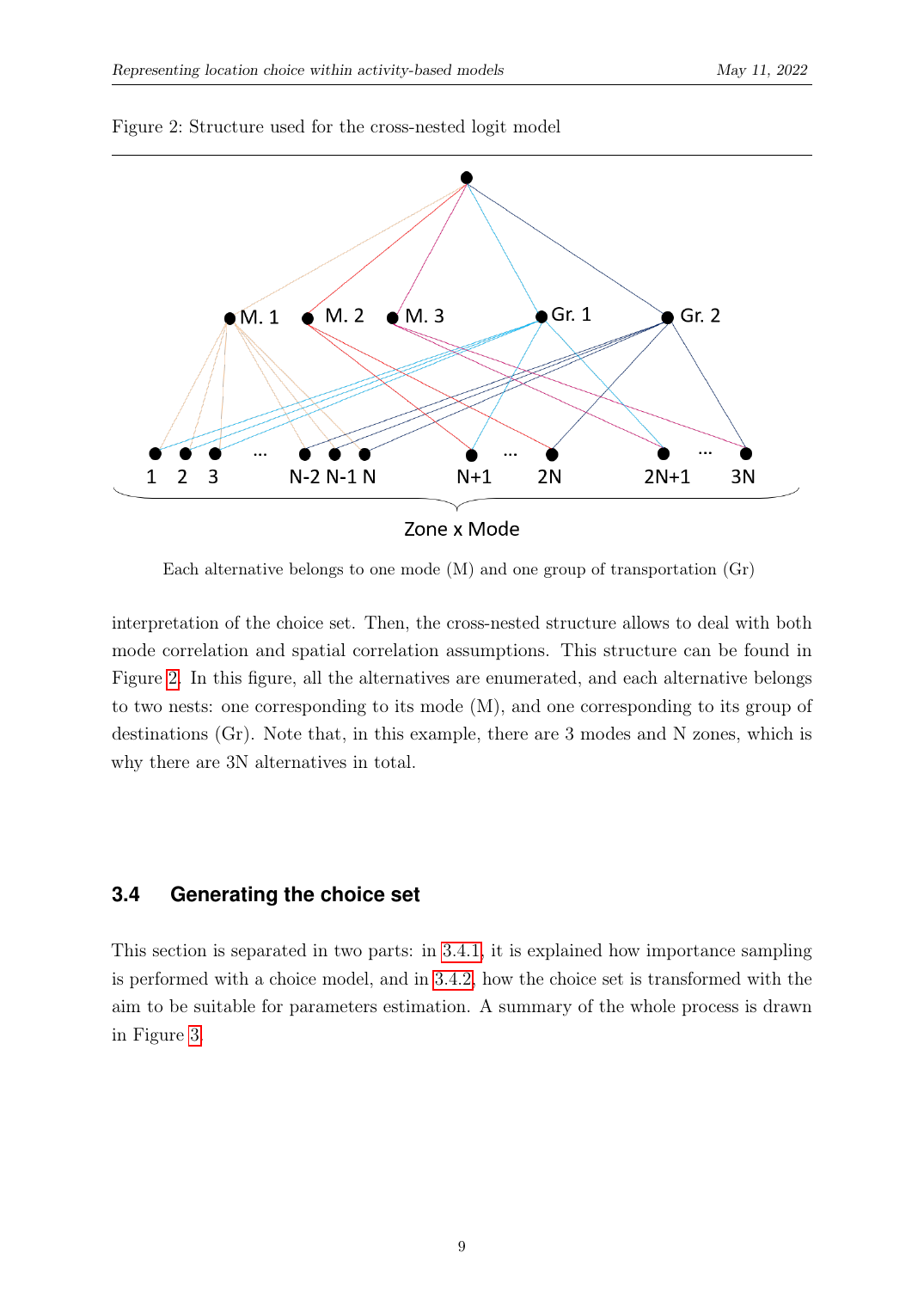
We estimate a cross-nested logit (CNL) on observed mode-and-destination combinations from a trip diary. The CNL structure puts every alternative into two nests simultaneously: one corresponding to its transportation mode (mode correlation between alternatives accessed the same way), one corresponding to its geographic group (spatial correlation between zones near the same amenity).

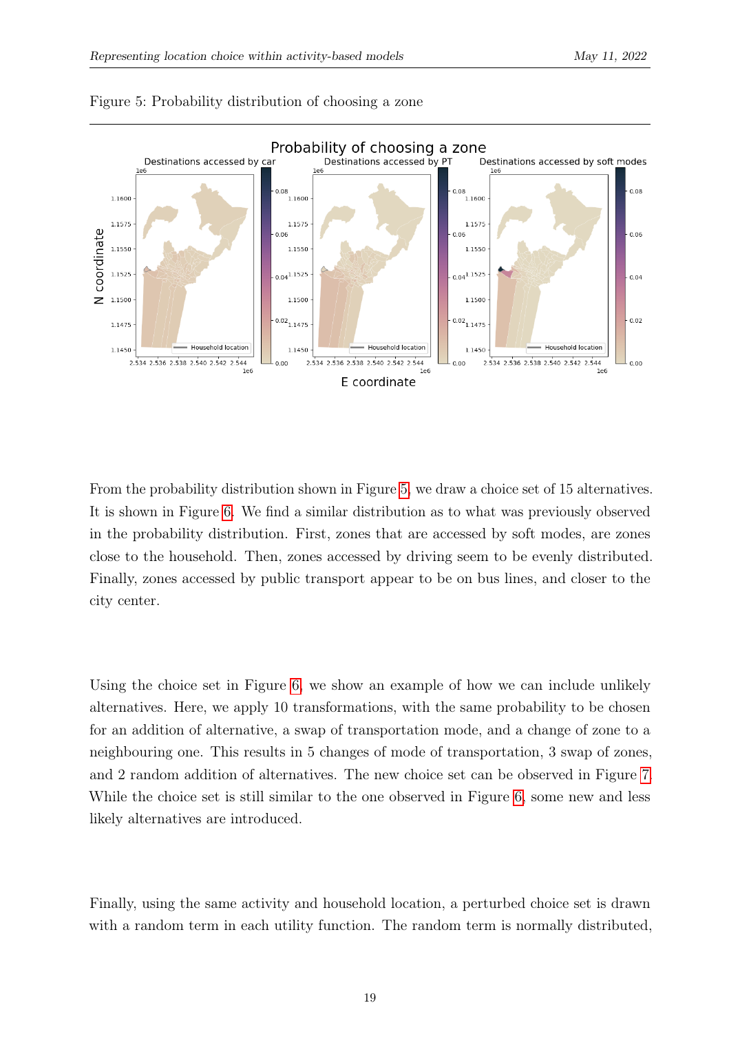
From the estimated CNL we importance-sample N alternatives per individual to form a choice set Ĉ_n. The probability of obtaining any specific choice set is closed-form, the product of per-draw probabilities adjusted for sampling-without-replacement, which means we can compute the correction term needed for unbiased maximum-likelihood estimation downstream.

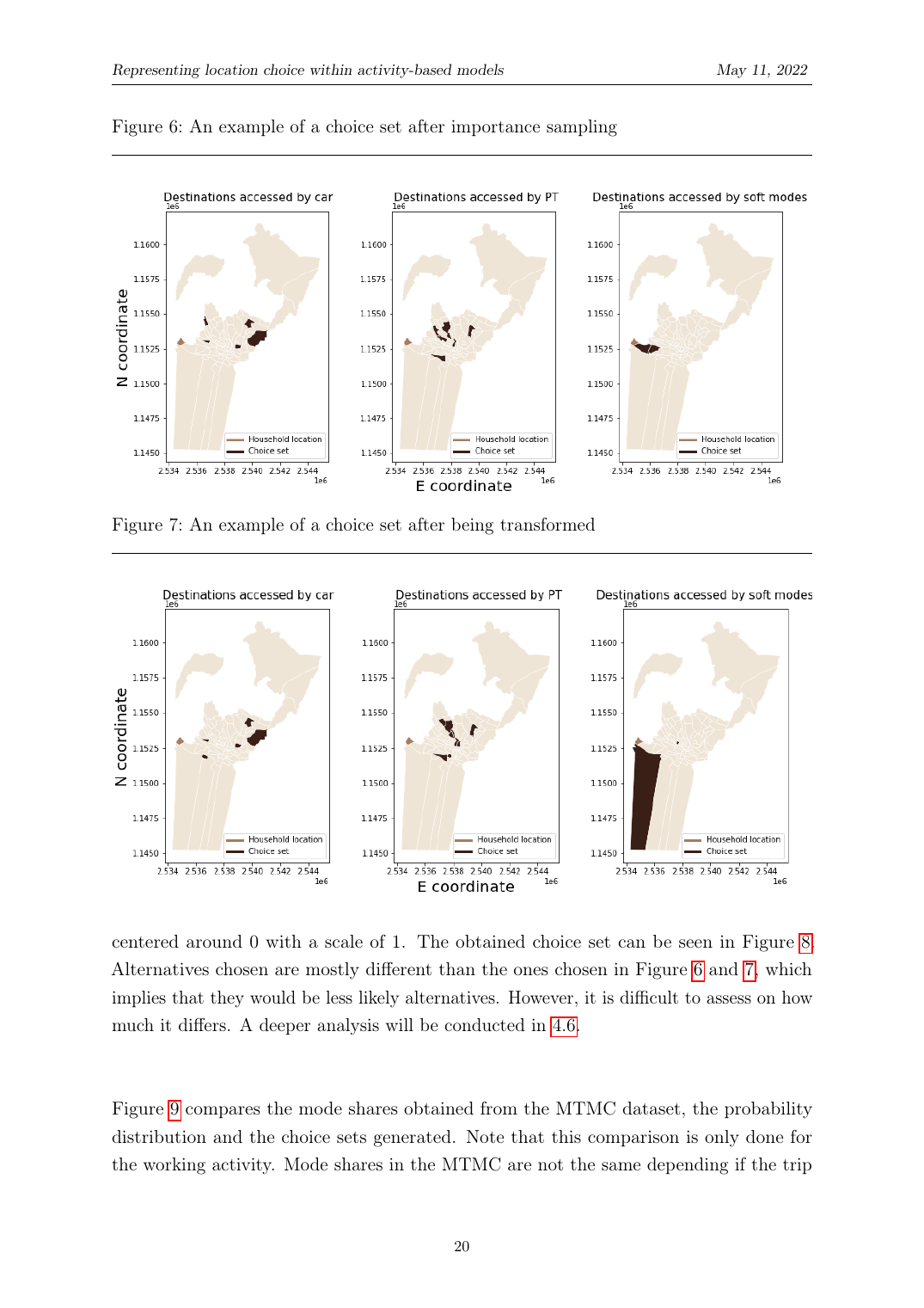
We perturb the importance-sampled set with three operators: (1) add a random alternative not in the set, (2) swap the mode of an alternative to a different mode, (3) shift the destination of an alternative to a neighboring zone. Each operator has a closed-form probability that contributes to the overall P(Ĉ_n) used in the bias-correction term. This injects the unlikely alternatives needed to identify why the chosen one is preferred.

We validated on the 2015 Swiss Mobility and Transport Microcensus, restricting to 3,536 trips with Lausanne destinations. The CNL fits significantly better than a simple logit on the same data (likelihood ratio 46.58, χ²(5, 95%) = 11.07, null rejected at high confidence).

The outcome

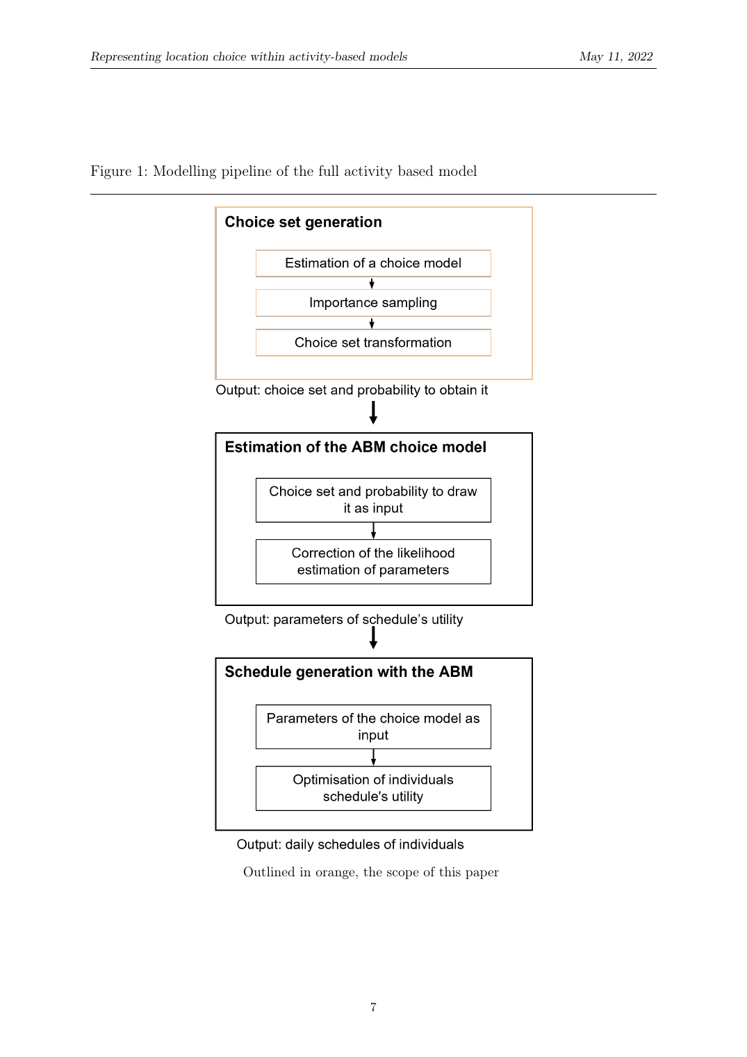
Deliverable: a methodology with a closed-form sampling probability P(Ĉ_n), which is what lets any downstream activity-based-model estimator add a single multiplicative correction term and recover unbiased parameter estimates. The choice-set generation now ships as the corresponding building block of the OASIS activity-based modeling pipeline at EPFL Transp-OR, presented at STRC 2022.

On the Lausanne case study (88 zones × 3 modes, 3,536 microcensus trips), the cross-nested logit fits significantly better than a simple logit (LR = 46.6 vs. χ²(5, 95%) = 11.07, null rejected at high confidence), confirming that the joint mode/destination coupling is real and worth modeling — not an assumption the prior generation of rule-based filters could capture.

Technical deep dive

The model behind the result.

The model

The methodological core has three pieces that fit together: a cross-nested logit specification for mode-and-destination utility, an importance-sampling rule that draws choice sets from the CNL probability distribution, and a perturbation step that injects unlikely alternatives while keeping the overall sampling probability closed-form. The closed-form sampling probability is the key, it's what lets the downstream activity-based-model estimator add a correction term and recover unbiased parameter estimates.

V_{z mn} = ASC_{m} + β_{m}^{TIME} \cdot T T_{z m} + β^{TYPE} \cdot T_{z} + a \sum ω_{a} \cdot β_{density}^{a} \cdot ρ_{z}^{a} .

Joint mode-and-destination utility. For individual n choosing zone z and mode m: an alternative-specific constant ASC_m per mode; a mode-specific travel-time coefficient β^TIME_m × TT_zm; a zone-type effect (urban/rural/intermediate); and an activity-dependent density effect ρ^a_z = job density, population density, or a sum, different for work, education, leisure, shopping, other. The activity-density coefficients let the model say things like 'a working activity prefers high-job-density zones' or 'an education activity prefers low-population-density zones' without losing the mode-destination coupling.

P_{n} (i ∣ C_{n}^{s}) = k = 1 \sum K \frac{( α _{ik} ) ^{μ_{k} / μ} e ^{μ_{k} V_{in}} ( \sum _{j \in C_{n}^{s}} ( α _{j k} ) ^{μ_{k} / μ} e ^{μ_{k} V_{j n}} ) ^{μ / μ_{k} - 1}}{\sum _{p = 1}^{K} ( \sum _{j \in C_{n}^{s}} ( α _{j p} ) ^{μ_{p} / μ} e ^{μ_{p} V_{j n}} ) ^{μ / μ_{p}}} .

Cross-nested logit choice probability. Each alternative i belongs to two nests simultaneously (a mode nest and a geographic-group nest), with degree-of-membership α_ik ∈ [0, 1]. The scaling parameters µ_k > 1 capture correlation within each nest, empirically estimated at 1.63 (PT) up to 7.06 (car) on the Lausanne data. The CNL fits significantly better than a simple logit (LR test 46.58 vs. χ²(5) = 11.07).

P_{IS} (C_{n}) = j = 1 \prod N \frac{P _{n} ( j )}{1 - \sum _{l = 1}^{j - 1} P _{n} ( l )} .

Importance-sampling probability without replacement. The probability of drawing a specific choice set Ĉ_n of size N is the product of N per-draw probabilities, numerator is the CNL choice probability of the j-th alternative, denominator re-normalizes after each previous draw is removed from the support. This is closed-form, which is the whole point: the downstream MLE knows P_IS exactly and can compute the bias-correction term without Monte Carlo integration.

P_{add} (j) = \frac{1}{Z M - N}, P_{swap} (j) = \frac{1}{N ( M - 1 )}, P_{change} (j) = \frac{1}{N \cdot Nei _{j}} .

Perturbation-operator probabilities. After importance sampling, three operators inject unlikely alternatives: 'add' picks a random alternative not in the set (uniform over the ZM − N alternatives outside Ĉ_n); 'swap' picks an alternative and swaps its mode (1/N to pick the alternative × 1/(M−1) to pick a different mode); 'change' shifts an alternative's zone to a random neighbor (1/N × 1/Nei_j where Nei_j is the number of geographic neighbors). Each is invalid when the resulting alternative is already in the set, handled by rejection.

P (C_{n}) = P_{IS} (C_{n}) \cdot t = 1 \prod T P_{t} (j_{t}), P_{t} (j) \in {p_{add} P_{add}, p_{swap} P_{swap}, p_{change} P_{change}} .

Overall sampling probability after T perturbations. The modeler picks the three operator-selection probabilities (p_add, p_swap, p_change summing to 1) and the number of perturbations T. The total probability P(Ĉ_n) is the product of the importance-sampling probability and the per-perturbation probabilities, still closed-form, which is what makes this whole construction usable in maximum-likelihood estimation downstream.

ln L_{corrected} (β) = n \sum ln \frac{e ^{V_{i_{n} n} (β)} / P ( i _{n} \in C _{n} )}{\sum _{j \in C_{n}} e ^{V_{j n} (β)} / P ( j \in C _{n} )} .

Corrected log-likelihood for downstream ABM estimation. With the per-alternative inclusion probability P(j ∈ Ĉ_n) known (computable from P(Ĉ_n)), the activity-based model's MLE can correct for the fact that we're estimating on a sampled choice set instead of the universal one. Without this correction term, the parameters are biased, alternatives that the sampler over-represents look more attractive than they really are. McFadden's classical result generalizes to this case because P_IS is closed-form.

L R = - 2 (L_{logit} - L_{CN-logit}) = - 2 (- 16755.54 + 16732.25) = 46.58 > χ^{2} (5, 95%) = 11.07.

Specification test: CNL vs. simple logit. The cross-nested structure has 5 more free parameters than the constrained-to-be-logit version (set all α to 0/1 and all µ to 1). Likelihood-ratio statistic of 46.58 vastly exceeds the χ² critical value at 95% confidence, the CNL structure is significantly better-fitting. Concretely: there is real mode correlation and real spatial correlation in the data, and modeling them improves the fit enough to warrant the extra parameters.

The closed-form P(Ĉ_n) is the load-bearing piece of the whole construction. Once you have it, all the downstream activity-based-modeling machinery, likelihood-based estimation, simulation under the estimated parameters, importance-sampled prediction, works correctly without needing to track which alternatives the sampler did or didn't see, because the bias correction lives in a single multiplicative factor. The CNL on top is the modeling choice that makes the joint mode-and-destination interaction explicit; without it (with a simple logit) the IIA property would force unrealistic substitution patterns whenever you add or drop alternatives.

Benchmark

Cross-nested logit estimation on the 2015 Swiss Mobility and Transport Microcensus (3,536 Lausanne trips, 88 zones × 3 modes, biogeme 3.2.6). Reported values are coefficient estimates with robust standard errors. ASC = alternative-specific constant; B_TIME = travel-time coefficient per mode; B_<x>_<activity> = density effect for activity type. The 5 µ parameters are the nest-scaling coefficients (must be > 1 to make sense; > 1 means within-nest correlation).

Parameter	Value	Robust std err	Robust t-test	Robust p-value
ASC_car	−1.99	0.118	−16.8	≈ 0
ASC_pt	−1.73	0.190	−9.12	≈ 0
B_TIME_softmodes	−0.537	0.0124	−43.3	≈ 0
B_TIME_car	−0.457	0.0818	−5.59	2.2e-08
B_TIME_pt	−0.327	0.0589	−5.55	2.9e-08
B_JobD_WORK	+0.00335	0.00136	+2.48	0.013
B_PopD_EDUC	−0.0251	0.00576	−4.36	1.3e-05
B_PopD_LEIS	−0.0189	0.00291	−6.51	7.3e-11
B_JobD_PopD_SHOP	+0.00712	0.00334	+2.13	0.033
MU_CAR (nest scaling)	7.06	4.99	1.41	0.157
MU_PT (nest scaling)	1.63	0.433	3.76	1.7e-04
MU_CENTER (geo nest)	1.66	0.118	14.1	≈ 0
MU_EAST (geo nest)	2.05	0.186	11.0	≈ 0
MU_WEST (geo nest)	1.98	0.177	11.2	≈ 0

Three substantive findings. First, the alternative-specific constants for car (−1.99) and public transport (−1.73) are both negative, meaning soft modes (walking/biking) are baseline-preferred when travel time and other factors are zero, consistent with the short trips in a 0.5–5 km Lausanne dataset. Second, the activity-density coefficients flip sign by activity: working activities prefer high-job-density zones (+0.0034 / job·m^−2), leisure and education activities prefer low-population-density zones (−0.019 to −0.025 / person·m^−2). This is exactly the substitution pattern a simple logit can't capture, different activities pull toward different parts of the city. Third, the geographic nest parameters (MU_CENTER = 1.66, MU_EAST = 2.05, MU_WEST = 1.98) are all significantly above 1, confirming real spatial correlation: zones inside the same group share unobserved characteristics that pull individuals toward them collectively. MU_CAR's high estimate (7.06) with marginal significance is a small-sample artifact (only 1,316 car trips with 276 alternatives apiece).

From the record

Figure 1 from the paper: the modeling pipeline of the full activity-based model. The scope of this work (outlined in orange) is the first stage, generating a choice set for each individual along with the closed-form probability P(Ĉ_n) of obtaining it. That probability propagates downstream as the bias-correction term in the ABM parameter estimation, and then through to the schedule-generation step that uses the estimated parameters.

Figure 2: the cross-nested logit structure. Each alternative (a zone × mode combination) belongs to two nests simultaneously: a mode nest (M_1, M_2, M_3 for soft modes / car / public transport) and a geographic-group nest (Gr_1, Gr_2 for spatial clusters of zones). The double-nesting captures both mode correlation (alternatives in the same mode share unobserved comfort/perception terms) and spatial correlation (alternatives in the same geographic cluster share unobserved attractor properties).

Figure 5: probability distribution of choosing a zone for a representative household in west Lausanne with a working activity, decomposed by mode. The soft-modes map (left) concentrates probability mass right around the household location, soft modes can't span the city. The car map (middle) is nearly uniform across zones, driving makes most destinations roughly equally accessible. The PT map (right) has sharp spikes along bus and tram lines, the public-transport network's geometry leaks directly into the choice probabilities.

Figures 6 and 7: an importance-sampled choice set of 15 alternatives (top) and the same set after 10 perturbations (bottom). The importance-sampled set looks 'too clean', every alternative is plausible under the estimated CNL. The perturbed set injects 5 mode swaps, 3 zone changes, and 2 random additions, producing the mix of likely-and-unlikely alternatives the downstream ABM needs to estimate parameters without bias. The chosen alternative is by construction always in the set.

Techniques

Cross-nested logit model (CNL)
Importance sampling for choice sets
Joint mode/destination probability distribution
Activity-based travel demand
Bias correction in DCM estimation
Stochastic perturbation operators

Stack

Python
Biogeme 3.2.6
Swiss Microcensus 2015
MATSim distance matrices

A problem like this?

We'd like to hear about it.

contact@optimally.ch