Constraint Programming, 750× Faster Than MILP on Activity-Based Scheduling
An idiomatic CP-SAT formulation, with the negative finding that NO_OVERLAP intervals are actively slower here, the kind of paradigm-choice judgment we deliver to clients
When everyone is using MILP, sometimes you switch paradigms. The team took the published MILP for activity-based scheduling from Pougala, Hillel and Bierlaire (2021), rebuilt it in constraint programming using OR-Tools' CP-SAT, and proved that idiomatic CP, implications as native constraints, ELEMENT global constraints, propagation instead of branch-and-bound, outperforms the MILP by 750× on 5-activity instances.
The deeper lesson, which is the value we deliver to clients: not every optimization problem deserves the same hammer. A negative finding too, interval variables and NO_OVERLAP, often advertised as CP-SAT's killer feature for scheduling, *don't* help here, because the time-consistency constraint already pins down activity sequencing.
The challenge
Activity-based scheduling under utility maximization (Pougala et al. 2021) is the modern econometric approach to travel-demand forecasting, it captures the joint trade-off across activity participation, timing, duration, location, and mode that older sequential rule-based ABMs miss. The price is a brutal MILP: full-population simulation runtime scales by roughly an order of magnitude per added activity per individual, which is unworkable when you need to simulate millions of agents.
The natural question, would a different solver paradigm fit the problem better?, was unanswered in the literature for activity-based scheduling specifically. Naïve translations between paradigms rarely help; the real question is whether *idiomatic* CP, using global constraints and propagation engines that exploit the discrete combinatorial structure, can outperform a refined MILP.
Our approach
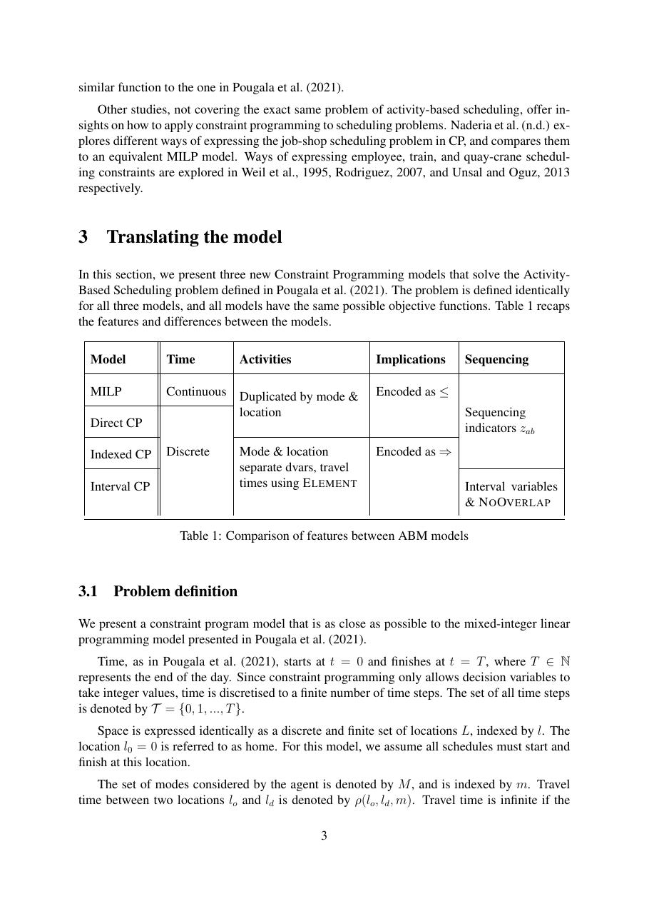
We co-supervised three CP variants of the Pougala et al. (2021) MILP, all implemented in Google OR-Tools' CP-SAT solver and benchmarked head-to-head against the original MILP. Time is discretized in the CP versions (CP requires integer decision variables) while the MILP keeps continuous time.
Variant 1, Direct CP translation: a near-mechanical port of the MILP. Same activity-duplication scheme (one decision variable per activity × mode × location triple, with sequencing indicators z_ab and α_a^car for tour mode consistency). Implications written as native CP constraints instead of being big-M-linearized. Used as the baseline 'what does CP do for free?'.
Variant 2, Indexed CP: replaces the activity duplication with array indexing. Mode m_a and location l_a become decision variables per activity (instead of having a separate copy of each activity for every combination); the travel-time lookup is done via the ELEMENT global constraint over a flattened |M| × |L|² travel-time array D. Mode consistency becomes a clean two-line implication. This is the version that wins.
Variant 3, Interval CP: adds CP-SAT's interval variables I(x_a, Θ_a, y_a, ω_a) with NO_OVERLAP across all activities. In theory this should help, interval scheduling is a CP-SAT showcase use case. In practice it doesn't, because the existing time-consistency constraint (z_ab ⟹ x_a + τ_a + t_ab = x_b) already pins activities into sequence, leaving NO_OVERLAP as redundant overhead.
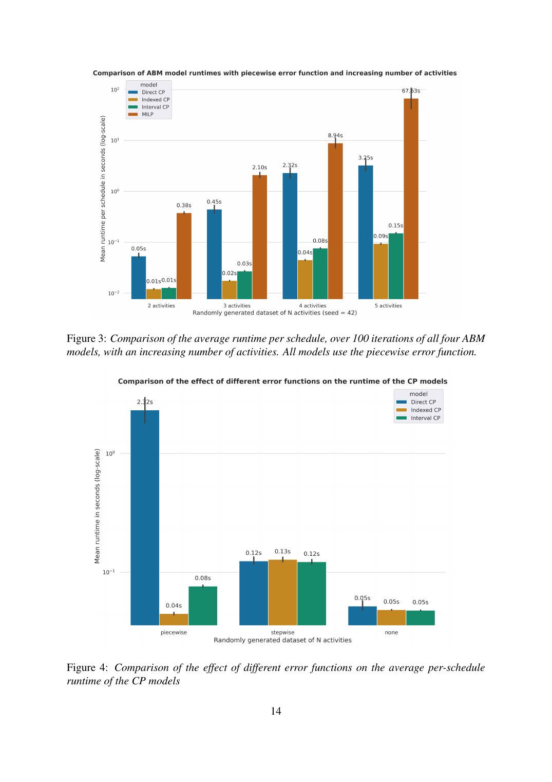
All variants were benchmarked on randomly generated activity sets from RANDOM-2 to RANDOM-5 (2 to 5 distinct activities, with dawn and dusk fixed). 100 iterations per (model, instance) pair, fresh error parameters each time, with bootstrapped 95% confidence intervals on the mean runtime.
The outcome
The indexed CP variant outperforms the MILP baseline by approximately one order of magnitude on 2-activity instances and by nearly three orders of magnitude on 5-activity instances. At 5 activities the MILP takes 67.6 s while the indexed CP takes 0.09 s, a 750× speedup. The direct CP translation alone buys 20× over the MILP at 5 activities, demonstrating that even a mechanical paradigm switch pays off here.
The deliverable is more than a runtime number: it is a methodology for choosing the right paradigm per problem class, and a clear negative finding (interval variables don't help) that prevents the team from over-promising CP-SAT's interval features on similar problems in the future.
Technical deep dive
The model behind the result.
The model
The activity-based scheduling problem from Pougala et al. (2021) generates a daily schedule for an individual: choose which activities to perform, in which order, at what start time, for how long, at which location, with which mode of transport, to maximize a utility function that penalizes deviation from the individual's desired schedule (early-/late-start penalties, short-/long-duration penalties, travel-time penalty). Each of the three CP variants below encodes the same optimization problem; the differences are how each variant chooses to express activity duplication and interval logic.
Shared utility objective. The deterministic penalty terms V depend on flexibility parameters per activity, how much the individual is willing to start early/late or do shorter/longer durations. The stochastic terms U are Gumbel(0, 1) errors (for the generic schedule-level taste U) plus per-activity error functions over duration, start time, mode, and sequencing. All four CP variants and the MILP optimize the same objective; the only differences are how they encode the feasibility constraints below.
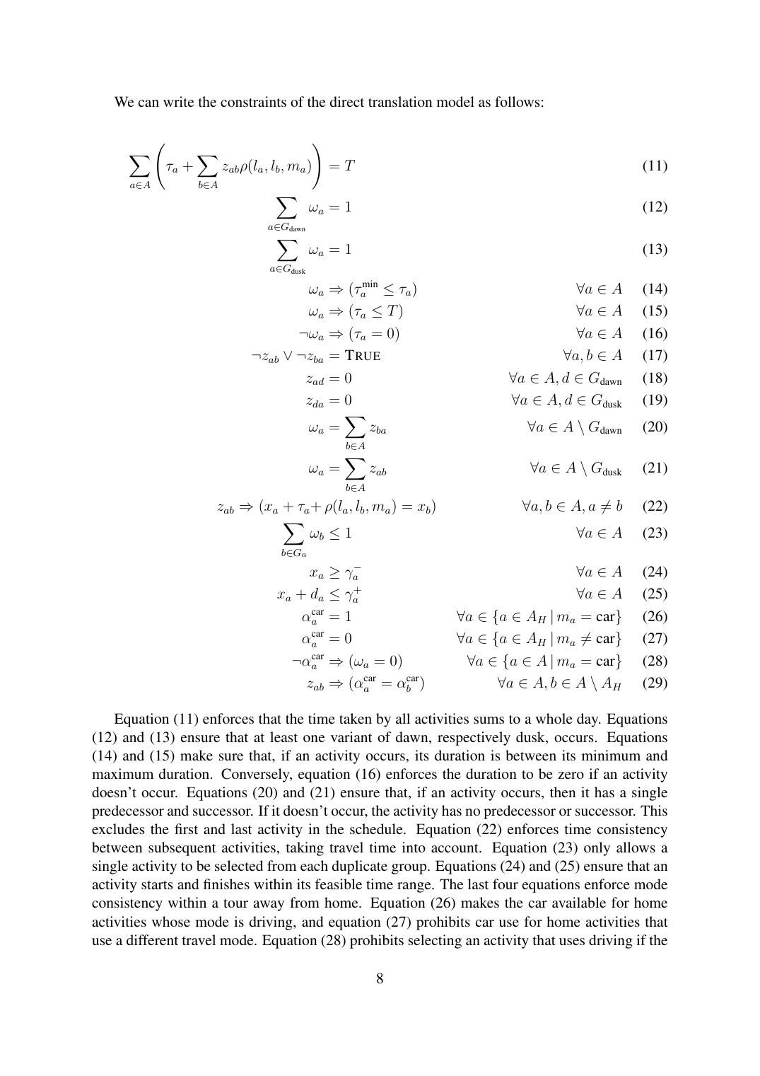
Full-day sum and sequencing. Total time spent on activities plus inter-activity travel must equal the day length T. The implication z_ab ⟹ (x_a + τ_a + ρ = x_b) is the key constraint that propagates start-time information along the chosen sequence. In the MILP this is big-M-linearized into two ≤ constraints; in CP it's a single native implication that CP-SAT's propagator handles directly, which is where a meaningful chunk of the speedup comes from.
Direct translation: keep MILP's activity-duplication trick. Each (location, mode) combination for an activity is a separate decision variable, with the group constraint Σ ω_b ≤ 1 saying that only one copy of any activity makes it into the schedule. This bloats |A| by a factor of up to |L_a| × |M|. The direct CP runs 20× faster than the MILP at 5 activities purely from CP-SAT's better handling of the implication constraints, no structural change.
Indexed reformulation: stop duplicating, start indexing. Mode m_a and location l_a become decision variables per activity (no duplication). Travel times for all (mode, source, destination) combinations are stored in a flattened array D of size |M| × |L|² + 1. The ELEMENT global constraint enforces t_ab = D[i_ab], where i_ab is the computed index into D. This is the structural change that buys the additional order of magnitude, CP-SAT's ELEMENT propagator is sharper than what the direct version exposes.
Mode consistency on tours away from home. Once activity duplication is gone (indexed version), the rule 'if you took the car to activity a and b is not at home, you must still have the car at activity b' becomes two clean implications instead of the MILP's tangled big-M conditional constraints. This is a representative example: every rule the MILP encodes via z_ab × continuous variables turns into a one-line CP implication.
Interval variables with NO_OVERLAP. Adds optional intervals (active only when ω_a = 1) and the CP-SAT NO_OVERLAP global constraint, which is the textbook way to express 'no two activities run simultaneously' in CP-SAT. The negative finding: this is 1.5–2× slower than the indexed version, because the existing time-consistency implication z_ab ⟹ (x_a + τ_a + t_ab = x_b) already pins each activity into sequence, leaving NO_OVERLAP redundant. The constraint is technically valid but actively harmful, it forces CP-SAT to track more state without unlocking new propagation.
Scaling. The MILP's runtime grows by ~10× per added activity (0.38 s → 67.6 s from N=2 to N=5). The indexed CP grows by only a factor of 9 across the entire range (0.01 s → 0.09 s), giving a 750× advantage at N=5. The advantage compounds: the deeper question raised in the conclusion is whether the gap is entirely paradigm (CP propagation vs. branch-and-bound) or partly time discretization (CP forces integer time, which shrinks the decision space). The team flags this as a future research question, and it matters, because if the speedup is mostly from discretization, the MILP could close some of the gap with its own discretization pass.
The headline result is the 750× speedup, but the *interesting* result is the negative finding on interval variables. CP-SAT's interval-and-NO_OVERLAP feature set is marketed as the killer combo for scheduling, and for job-shop scheduling it absolutely is. But on this activity-based scheduling problem the existing time-consistency implication already does the work NO_OVERLAP would do, so adding the interval layer is pure overhead. Three lessons for client work: (1) paradigm choice matters more than parameter tuning when the problem structure aligns with one solver's strengths, (2) idiomatic rewrites beat direct translations by another order of magnitude after the paradigm swap, (3) flashy features aren't free, sometimes they're slower than the boring formulation that already works.
Benchmark
Mean solve time per schedule on randomly generated activity datasets (RANDOM-2 through RANDOM-5), 100 iterations per (model, dataset) pair with fresh error parameters each iteration, piecewise error function in the objective. Times in seconds. All four models recover schedules of comparable quality (objective values within noise), the differences are purely in runtime.
| # Activities | MILP | Direct CP | Indexed CP | Interval CP | Indexed / MILP speedup |
|---|---|---|---|---|---|
| 2 | 0.38 s | 0.05 s | 0.01 s | 0.01 s | 38× |
| 3 | 2.10 s | 0.45 s | 0.02 s | 0.03 s | 105× |
| 4 | 8.94 s | 2.32 s | 0.04 s | 0.08 s | 224× |
| 5 | 67.6 s | 3.25 s | 0.09 s | 0.15 s | 751× |
The MILP scales like ~10× per added activity, a textbook branch-and-bound explosion as the decision tree grows. The direct CP translation flattens after 3 activities (it benefits from CP-SAT's propagation engine but inherits the activity-duplication bloat). The indexed CP achieves nearly flat scaling: 0.01 → 0.09 s across the full range, a 9× growth for 2.5× more activities. The interval CP is consistently 1.5–2× slower than indexed, the negative finding. The cross-dataset gap widens fast: from 38× at the smallest instance to 751× at the largest. On a separate axis (objective function complexity), the piecewise error function exposes the largest CP-internal gap: direct = 2.32 s vs. indexed = 0.04 s vs. interval = 0.08 s at N = 5. With the zero or stepwise error function all CP variants finish in ~0.05–0.12 s, the complexity advantage of the indexed version only materializes under realistic objective shapes.
From the record
![Section 3.4, the indexed reformulation. Travel-time array D is flattened to size |M||L|² + 1; the index i_ab = |L|² m_a + |L| l_a + l_b is computed from the decision variables m_a, l_a, l_b; ELEMENT(i_ab, D, t_ab) enforces t_ab = D[i_ab]. This is the structural change that buys an additional order of magnitude over the direct translation. Mode consistency becomes a clean two-line implication (eqs 49–52) rather than the tangled big-M conditionals the MILP needs.](/figures/comparative/p-10.png)
Techniques
- Constraint programming with CP-SAT
- Mixed-integer programming (MILP baseline)
- ELEMENT global constraint
- Implication constraints as first-class objects
- Optional interval variables + NO_OVERLAP
- Time discretization for CP compatibility
Stack
- Python
- Google OR-Tools CP-SAT
- CPLEX (MILP baseline)
- Pougala et al. 2021 MILP
A problem like this?