← Areas of expertise/Revenue Management/2025

Exact Choice-Based Pricing, Up to 1.67 Million Times Faster Than the MILP Baseline

A spatial Branch-and-Benders algorithm + a polynomial-time Breakpoint Exact Algorithm that solves 1,000,000 demand scenarios in 77 seconds and beats the previous ML-specific state-of-the-art (CoBiT) by 300×

Pricing under modern demand models, mixed logit, nested logit, anything richer than a sales-101 spreadsheet, has been an algorithmic dead-end for decades. The textbook MILP formulation buckles past two prices. The state of the art conceded that 'exact' was simply out of reach.

Our work changed that. Published in OR Spectrum, our spatial Branch-and-Benders Decomposition and Breakpoint Exact Algorithm beat Gurobi's MILP solver by orders of magnitude, and our complexity result delivers a polynomial-time scheme in the customer and draw count.

1.67 × 10⁶ ×

speedup over Gurobi MILP on one-price optimization at R = 5,000 scenarios

1,000,000

demand scenarios solved in 77 seconds by the Breakpoint Exact Algorithm

300×

faster than CoBiT, the previous state-of-the-art for ML-specific pricing

OR Spectrum

peer-reviewed and published, Haering et al. 2024

The challenge

Choice-based pricing, choosing prices that maximize revenue when demand is generated by a discrete-choice model derived from random utility theory, is fundamental to airlines, hotels, retailers, and parking operators. Yet the existing exact formulation, the simulation-based MILP from Paneque et al. (2021), scales exponentially in the number of price draws.

Standard solvers crawl past trivial sizes; specialized heuristics work only for restricted demand specifications. There was no general, exact algorithm for the problem.

Our approach

We reformulated the canonical MILP into a non-convex Quadratically Constrained Quadratic Program with linear objective (QCQP-L), exposing structure that the MILP buries. We then designed a custom spatial Branch-and-Bound that uses McCormick envelopes for tight relaxations and branches by maximal violation rather than longest edge.

We accelerated each B&B node with Benders decomposition, so that the costly part of the relaxation is solved by a sequence of cheap sub-problems instead of one monolithic LP. The full pipeline is what we call B&BD, spatial Branch-and-Benders Decomposition.

We then exploited the piecewise-constant structure of choice probabilities along the price axis to develop the Breakpoint Exact Algorithm (BEA), whose complexity is polynomial in the number of customers and simulation draws (and exponential only in the number of priced products), making it the algorithm of choice when the price dimension is small.

The outcome

Deliverable: three exact algorithms for continuous choice-based pricing under any DCM with linear-in-price utility (mixed logit, nested logit, probit, paired combinatorial logit, anything in the family), plus a complete benchmark on the Ibeas et al. (2014) parking case study with mixed-logit demand. The Breakpoint Exact Algorithm solves 1,000,000 demand scenarios in 77 seconds, where Gurobi's QCQP-L reformulation takes 83,651 seconds at just R = 5,000 scenarios — a 1.67-million-× speedup. The Branch-and-Bound and Branch-and-Benders variants dominate when three or more prices are optimized simultaneously, with up to 20× speedup over Gurobi at four prices.

Versus CoBiT (Marandi and Lurkin 2023), the published state-of-the-art for ML-specific pricing, our methods are on average 42× faster (B&B), 8× faster (B&BD), and 300× faster (BEA) on two-price instances. CoBiT is hand-built for mixed logit; our methods work on any DCM with linear-in-price utility — and the broader applicability does not cost runtime, it gains it. Published in OR Spectrum, Haering et al. 2024.

Technical deep dive

The model behind the result.

The model

The problem is to set J controlled prices to maximize expected revenue when N customers choose among J + K alternatives under random-utility-derived demand. For modern DCMs (mixed logit, probit, nested logit), the choice probabilities have no closed form, so Paneque et al. (2021) approximated them by drawing R Monte Carlo scenarios of the error terms, freezing each draw into a deterministic utility, and writing a giant simulation-based MILP. The catch: every (i, n, r) tuple introduces a bilinear product pᵢ ωᵢₙᵣ between the price and the binary choice indicator, which the MILP linearizes with big-M auxiliaries, and the model blows up exponentially in R. Our chain of reformulations strips that structure out.

U_{in r} = c_{in r} + β_{p}^{in} p_{i}, ω_{in r} = 1 [U_{in r} = j \in C_{n} max U_{j n r}], P_{n} (i) \approx \frac{1}{R} r \sum ω_{in r} .

Simulation framework. For each Monte Carlo draw r ∈ {1, …, R}, customer n's utility for product i is a deterministic constant c_inr plus a price-linear term β_p · p_i. The choice variable ω_inr is 1 iff product i wins the arg-max for that (n, r). Averaging ω over the R draws gives an unbiased estimator of the true choice probability, and it converges to the underlying ML/probit/NL demand as R → ∞.

p, ω, U, h max \frac{1}{R} r \in R \sum n \in N \sum i \in C_{n} \sum p_{i} ω_{in r} s.t. ω \in {0, 1}^{(J + 1) N R}, KKT for each (n, r) .

Paneque et al.'s MILP (Formulation 4). The objective is the expected revenue. Constraints enforce that the choice variables ω solve a per-(n, r) utility-maximization knapsack, encoded via strong duality (primal feasibility + dual feasibility + complementarity). The bilinears p_i · ω_inr in the objective are linearized with big-M auxiliaries η_inr, that linearization is what destroys the knapsack's total-unimodularity and forces the problem to grow exponentially in R.

ω \in [0, 1]^{(J + 1) N R}, η_{in r} = p_{i} ω_{in r}, (QCQP-L, Formulation 6).

Our first reformulation. Drop the integrality on ω (the per-(n, r) knapsack is totally unimodular, so the LP relaxation is integral whenever utilities are distinct) and keep the bilinear η_inr = p_i ω_inr as an explicit non-convex quadratic equality. Result: a non-convex QCQP with linear objective. All non-convexity is now isolated in a single block of bilinear constraints, the rest of the model is linear.

η_{in r} \geq p_{i}^{L} ω_{in r}, η_{in r} \leq p_{i}^{L} ω_{in r} + p_{i} - p_{i}^{L}, η_{in r} \geq p_{i}^{U} ω_{in r} + p_{i} - p_{i}^{U}, η_{in r} \leq p_{i}^{U} ω_{in r} .

McCormick envelope. Replace each bilinear equality η_inr = p_i ω_inr by four linear inequalities valid over the current box [p_i^L, p_i^U] × [0, 1]. This is the tightest linear convex relaxation of the bilinear; tighter as the box shrinks. The resulting LP (Formulation 7) gives an upper bound on the QCQP-L revenue at each B&B node.

branch_index = ar g i \in {1, \dots, J} max n, r \sum \overset{η}{ˉ}_{in r} - \overset{p}{ˉ}_{i} \overset{ω}{ˉ}_{in r} .

Custom branching rule. Instead of longest-edge branching (textbook spatial B&B), we branch on the price whose bilinear constraint is most violated on average over (n, r) at the current relaxation solution. Empirically this dominates longest-edge, market-share-weighted, and random branching across every instance class we tested. We branch only on the J price variables, never on the JNR η or ω, which collapses the search tree by orders of magnitude vs. what Gurobi does on the raw QCQP-L.

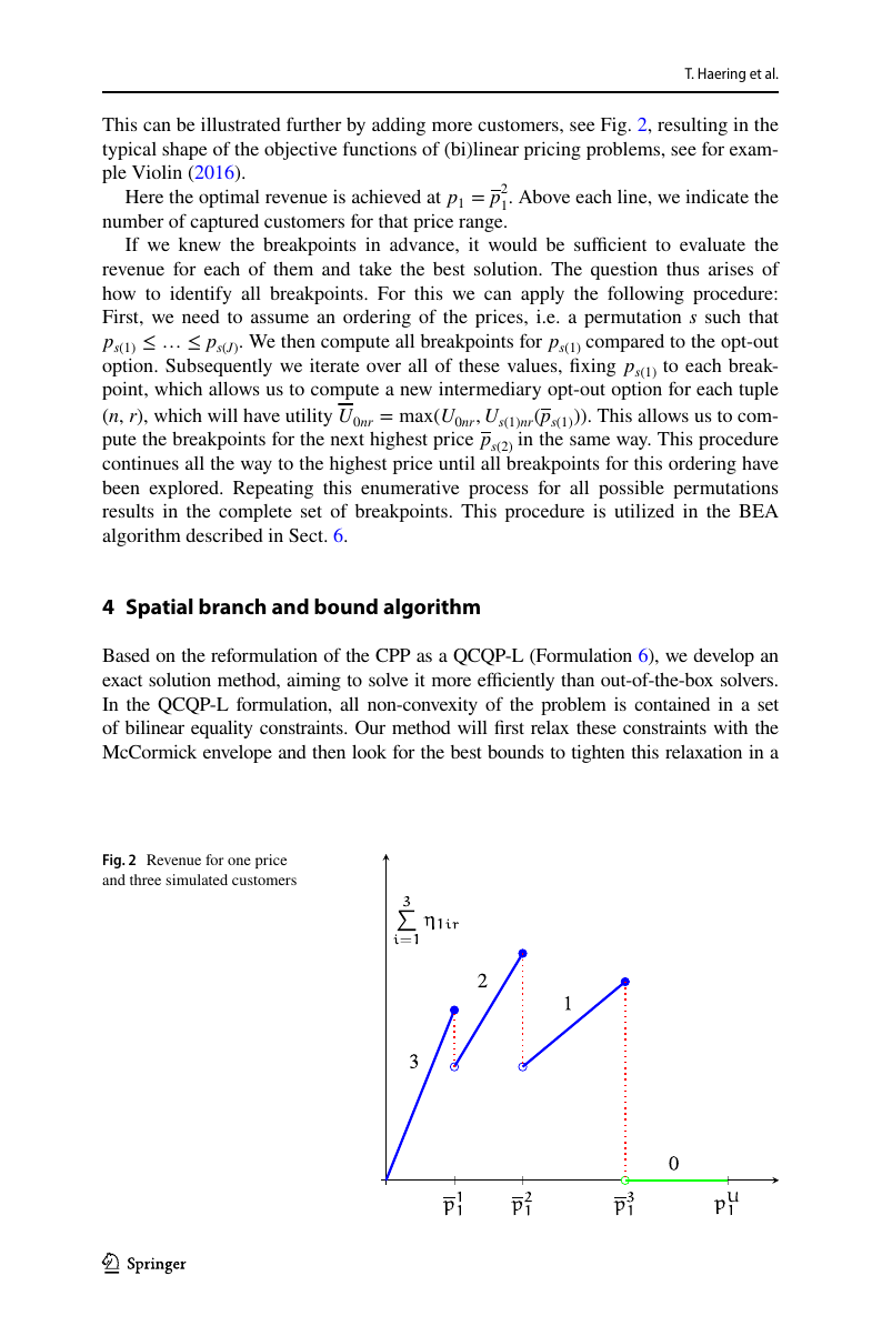
p_{i}^{⋆} \in {\frac{c _{0 n r} - c _{in r}}{β _{p}^{in}} : n \in N, r \in R} \cup {p_{i}^{L}, p_{i}^{U}}, ∣ B_{i} ∣ \leq N R + 2.

Breakpoint structure. At any optimal price p_i*, some customer n in some scenario r must be exactly indifferent between alternative i and the next-best option, otherwise we could raise p_i by ε without losing anyone. Solving the indifference equation gives the at-most-NR + 2 candidate prices per product (the box endpoints included). Enumerating across J products gives the search tree the BEA explores.

T_{BEA} (N, R, J) = O ((N R)^{J}) - polynomial in N, R; exponential only in J .

BEA complexity. The first polynomial-time-in-(customers, draws) algorithm for the choice-based pricing problem. For one or two priced products this is dramatically faster than any branch-and-bound, the BEA solved the one-price problem at one million draws in 77 seconds; Gurobi's QCQP-L formulation timed out at 7,000 draws after a full day. For three or more priced products, the J in the exponent makes the BEA blow up, and the B&B / B&BD approach wins.

Three algorithms, one paper. The Spatial B&B with custom branching beats Gurobi-on-the-MILP and Gurobi-on-the-QCQP-L by a clean order of magnitude. Adding Benders decomposition at each node (B&BD) projects out the JNR η and ω variables, which matters more the larger the instance: it pulls ahead of the plain B&B at 500 draws for four prices, at 1,000 draws for two prices, and at 3,000 draws for one price. The BEA dominates everything when J ≤ 2 because the breakpoint structure is enumerable; B&B / B&BD dominate when J ≥ 3 because the breakpoint tree is exponential in J. The right algorithm depends on the price dimension, and our paper makes the choice explicit, with the supporting complexity result.

Benchmark

Two-price optimization on the Ibeas et al. (2014) parking case study (J = 2, N = 50 customers, varying R = number of simulation draws). All times in seconds, 0.01% optimality tolerance, 72 h time limit, Gurobi 10.0.3 with hyperparameter tuning. All five methods recover the same optimal prices p₁ ≈ 0.56 and p₂ ≈ 0.67 with revenue ≈ 27.0.

Draws R	MILP (Paneque)	QCQP	QCQP-L	B&B (ours)	B&BD (ours)	BEA (ours)
200	9,042	4,195	3,403	1,386	3,015	11
300	42,804	9,503	7,951	2,998	5,418	24
400	112,335	22,567	19,283	6,378	11,858	41
500	242,877	32,886	25,030	7,963	12,064	69

The MILP scales catastrophically with the number of draws, from 2.5 hours at R = 200 to 67.5 hours at R = 500, a 27× runtime explosion for 2.5× more draws. The continuous reformulation (QCQP, QCQP-L) already buys a factor of 5–9 by removing the big-M tax. Our Spatial B&B with custom branching beats the MILP by ~30× across the board; the B&BD trades some of that lead for an overhead that pays off only at larger scales. The BEA is in a different league: at R = 500 it finds the proven optimum in 69 seconds versus the MILP's 242,877 seconds, a 3,520× speed-up. The story gets more dramatic at larger R: at 5,000 draws the BEA solves in 0.05 seconds where Gurobi's QCQP-L takes 83,651 seconds (a 1.6 × 10⁶ × factor); at 1,000,000 draws the BEA still finishes in 77 seconds.

From the record

Formulation 4 from the paper: the Paneque et al. (2021) simulation-based MILP, the previous state of the art. The bilinear products p_i · ω_inr in the objective and in the ζ_nr constraints are what hurt: linearizing them with big-M auxiliaries breaks the per-customer knapsack's total-unimodularity, which is why the model size and runtime both blow up exponentially in R.

Formulations 5 and 6: our two-step reformulation. Form. 5 (QCQP) drops the integrality on ω and keeps the bilinear p_i · ω_inr inside the constraint ζ_nr, exploiting that the LP relaxation of the knapsack is already integral under distinct utilities. Form. 6 (QCQP-L) then introduces η_inr = p_i · ω_inr as an explicit bilinear equality constraint and pulls all non-convexity into one block, the only thing the spatial B&B has to branch on.

Figure 3 and Formulation 7 from the paper: the spatial B&B tree (top) and the McCormick LP relaxation solved at each node (bottom). Each subproblem inherits a tighter box [p̂_i^L, p̂_i^U]; the McCormick inequalities λ¹ – λ⁴ replace the bilinear η_inr = p_i ω_inr with the tightest linear convex hull over the current box. We branch only on the J price variables (not on the JNR η or ω), which is what keeps the tree manageable as instance size grows.

Figure 1 from the paper (inset): the staircase shape of the revenue function in a single price for a single simulated customer. The revenue jumps at the price where the customer becomes indifferent between the priced product and the opt-out. With N customers and R draws there are at most NR such jumps, the BEA exploits this discrete structure to find the global optimum by enumerating those breakpoints in polynomial time.

Techniques

Spatial Branch-and-Bound
Benders decomposition
McCormick envelope relaxations
Breakpoint enumeration
Random utility / DCM modeling

Stack

Python
Gurobi 10
Julia (CoBiT comparison)
Discrete choice modeling stack

A problem like this?

We'd like to hear about it.

contact@optimally.ch