← Areas of expertise/Discrete Choice · Estimation/2025

BHAMSLE: +17.2% Log-Likelihood Lift on London Mode-Choice Mixture, in Half the Runtime of Multistart Biogeme

A Breakpoint Heuristic Algorithm for Maximum Simulated Likelihood Estimation of advanced discrete-choice models — exploits the same combinatorial structure that powered our OR Spectrum pricing algorithms

Estimating modern latent-class and discrete-continuous mixture choice models is a quiet computational nightmare. Hundreds of local maxima, simulation noise, and likelihood surfaces that look like the Alps. Standard solvers find a peak, usually the wrong one.

We took the breakpoint structure we discovered for choice-based pricing and ported it across to the estimation problem. The result, BHAMSLE, finds higher log-likelihoods, more interpretable latent segments, and better recovery of true parameters than CMA-ES, the existing MILP-based estimator, and even multistart Biogeme with 50 random restarts.

+17.2%

log-likelihood lift on the London mode-choice discrete-continuous mixture

Half the runtime

of Multistart Biogeme M=20, which is the minimum restart count that matches the BHAMSLE solution

7.7×

faster than Multistart Biogeme M=100 at identical final log-likelihood

Recovers truth

latent class split (0.69, 0.31) where default Biogeme stays stuck at uniform (0.50, 0.50)

The challenge

Maximum simulated likelihood estimation of advanced DCMs, latent-class models with continuous mixtures, restricted choice sets, and flexible utility specifications, is plagued by multimodality and simulation-induced noise. The likelihood surface of even a two-class logit can show several distinct high-likelihood basins; Newton-type estimators converge to whichever one happens to be closest to the starting point.

The only structure-aware approach in the literature is the Fernández Antolín (2018) MILP reformulation, which guarantees global optimality in principle but doesn't scale past tiny instances. Standard practitioner workarounds, multistart from random initializations, CMA-ES, PSO, pay for the multimodality with brute force, and routinely converge to interpretable nonsense (one class with 100% probability, zero-variance 'distributions', collapsed mixed parameters).

Our approach

We observed that simulation-based MSLE shares the same combinatorial backbone as choice-based pricing: per-individual indicator variables ω_inr that switch at finitely many parameter-dependent breakpoints, with the objective (log-likelihood here, revenue there) piecewise-constant between switches.

On that observation we built BHAMSLE: a coordinate-ascent algorithm that walks the parameter space breakpoint by breakpoint, evaluating the simulated log-likelihood exactly at each switch, exploiting structure that CMA-ES, PSO, and gradient methods are oblivious to. Two breakpoint sources are handled separately: utility-parameter breakpoints (where ω flips as β changes, given fixed class assignment) and scoring-function breakpoints (where class membership itself flips as α or γ changes).

BHAMSLE is positioned not as a final estimator but as an initialization strategy: drop it in front of Biogeme's standard Newton-type routine and watch the final solution improve, with the structure-exploiting search costing minutes instead of the hours that multistart Biogeme needs.

The outcome

Deliverable: BHAMSLE, a breakpoint-heuristic initialization scheme for Maximum Simulated Likelihood Estimation of advanced discrete-choice models (latent classes, continuous mixtures, discrete-continuous mixtures). The method exploits the same combinatorial structure that powered our OR Spectrum pricing algorithms, applied here to log-likelihood instead of revenue.

On the London mode-choice discrete-continuous mixture (N = 500, R = 500), Biogeme initialized with BHAMSLE reaches LL = −243.68 versus −294.38 with default initialization, a +17.2% improvement, in 3.8 hours. Multistart Biogeme needs 20 restarts (7.4 hours, roughly 2× the BHAMSLE runtime) to match this; with 100 restarts, it takes 7.7× the BHAMSLE runtime for the same final quality. On the discrete latent-class test, BHAMSLE-initialized Biogeme recovers the true class split (0.69, 0.31) where default Biogeme stays stuck at uniform (0.50, 0.50).

Technical deep dive

The model behind the result.

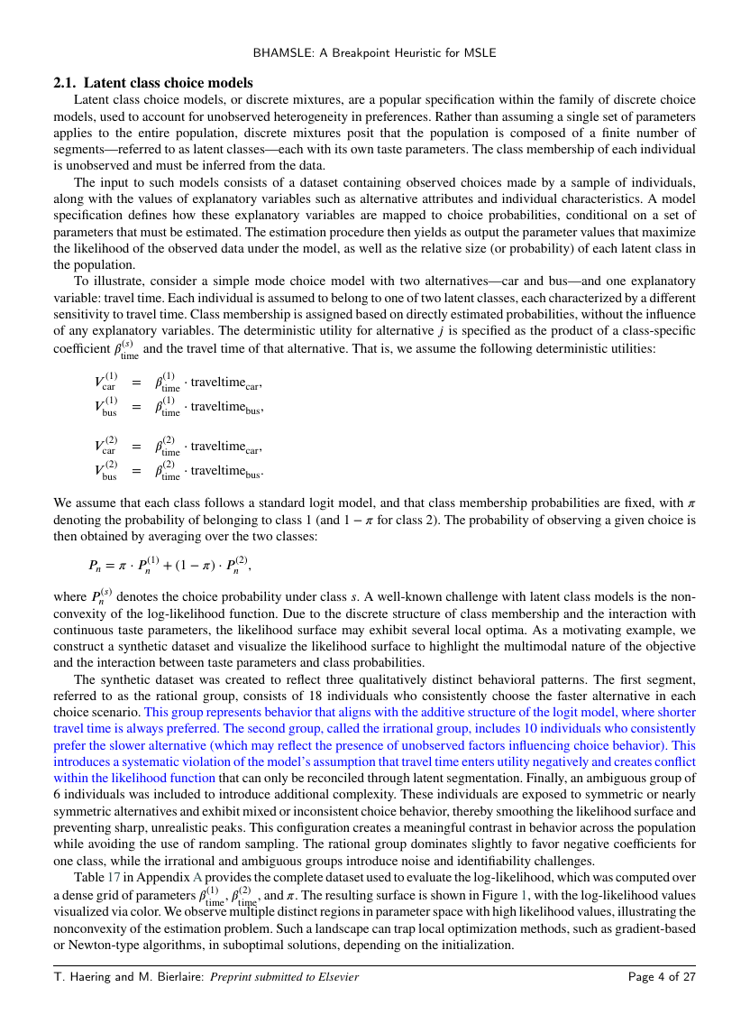
The model

Maximum simulated likelihood estimation of an advanced DCM has a fundamentally different structure than the textbook logit. The choice probabilities have no closed form (mixture models integrate over continuous distributions of taste parameters), so we approximate them by Monte Carlo. That introduces R simulated scenarios per individual, and at every parameter value, each (n, r) pair has a deterministic 'observed alternative wins' indicator that flips on or off based on whether the parameter is above or below a customer-scenario-specific threshold. The breakpoint structure that BHAMSLE exploits is exactly the set of parameter values at which one of those flips happens.

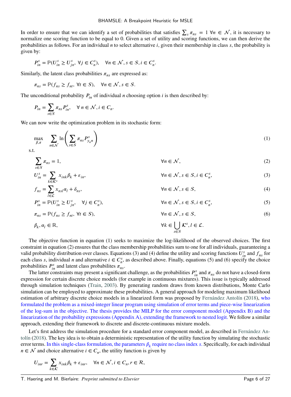
β, π max n \in N \sum ln (s \in S \sum π_{n s} P_{y_{n} n}^{s} (β)), P_{in}^{s} = P (U_{in}^{s} \geq U_{j n}^{s} \forall j \in C_{n}^{s}) .

The MSLE problem in its stochastic form. Sum over individuals of the log of a probability-weighted average of per-class choice probabilities. The decision variables are the utility coefficients β (often class-dependent) and the class membership probabilities π. For continuous mixtures, P^s_in is an integral over a normal density of distributed taste parameters, which is why simulation is needed.

U_{in r}^{s} = k \in K_{s} \sum x_{ink} β_{k} + ε_{in r}, ω_{in r}^{s} = 1 [U_{in r}^{s} = j \in C_{n}^{s} max U_{j n r}^{s}] .

Simulation framework. For each scenario r and individual n, the utility of alternative i under class s becomes deterministic once the error term ε_inr is drawn. The choice indicator ω^s_inr is 1 iff i wins the arg-max for that (n, s, r). Averaging ω over the R draws gives an unbiased estimator of P^s_in (Train 2003).

s LL (β, π) = - N ln R + n \in N \sum ln (Σ_{n} (β, π)), Σ_{n} := r \in R \sum s \sum 1_{class assignment} \cdot ω_{y_{n} n r}^{s} .

Simulated log-likelihood after Monte Carlo. Σ_n counts how many of the R scenarios pick the observed alternative y_n for individual n (under that scenario's class assignment). The objective is the sum of log-Σ_n over individuals, a piecewise-constant function of β and π, jumping at every breakpoint where some ω switches.

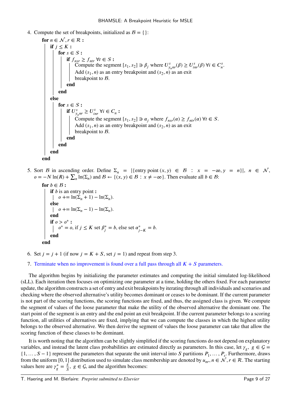
[s_{1}, s_{2}] : U_{y_{n} n r}^{s} (β_{j}) \geq U_{in r}^{s} (β_{j}) \forall i \in C_{n}^{s} . (entry breakpoint s_{1}, exit breakpoint s_{2})

Breakpoint construction for a utility parameter β_j. Freezing all other parameters, the segment of β_j for which the observed alternative y_n remains dominant for individual n in scenario r under class s is bounded by two indifference points. The lower bound s_1 is an 'entry' breakpoint (ω flips on as β_j increases past it); the upper bound s_2 is an 'exit' (ω flips off). Across all (n, r, s) we get at most 2NRS breakpoints per parameter.

At an entry breakpoint: Δ s LL = ln (Σ_{n} + 1) - ln (Σ_{n}); at an exit: Δ s LL = ln (Σ_{n} - 1) - ln (Σ_{n}) .

Incremental log-likelihood updates. Walking the breakpoints in sorted order along the j-th coordinate, the change in the simulated log-likelihood at each one is just the difference of two log-counts, O(1) work per breakpoint, vs. the O(NR) cost a black-box optimizer would pay to re-evaluate the full objective. This is what makes BHAMSLE scale: one full coordinate sweep costs O(NRS) instead of O((NR)²) for naive line search.

β_{j}^{(t + 1)} = ar g β_{j} \in B_{j} (β_{- j}^{(t)}) max s LL (β_{- j}^{(t)}, β_{j}), j (t + 1) = (j (t) mod (K + S)) + 1.

BHAMSLE outer loop. Coordinate ascent over the K utility parameters and the S − 1 class-probability parameters. At each step we freeze K + S − 2 parameters, enumerate the breakpoints for the active coordinate, and pick the breakpoint that maximizes the simulated log-likelihood. Terminate when a full K + S coordinate pass produces no improvement above τ = 10⁻⁶.

T_{BHAMSLE} = O (C \cdot (K + S) \cdot N R S) ≪ T_{Multistart Biogeme} = O (M \cdot T_{Newton}) .

Complexity comparison. C is the number of outer coordinate-ascent cycles (empirically < 20 on benchmark instances); the inner term NRS is the breakpoint enumeration and incremental update. Multistart Biogeme has to pay a full Newton convergence per restart M, and M needs to grow with the number of local optima, which for discrete-continuous mixtures is in the hundreds. On the Test 4 London mixture, BHAMSLE matches multistart Biogeme at M = 20 in roughly half the wall-clock time and outperforms M = 10.

What we did here is take a structural observation from a totally different problem class, pricing, and notice it carries across to estimation, because both problems compute an outer objective over simulated discrete-choice indicators. The same breakpoint enumeration that drove BEA and BHA in the pricing papers drives BHAMSLE here, with two new wrinkles: (1) the objective has a log instead of a sum, which means we use incremental ln-updates instead of additions, and (2) the latent-class parameters live inside indicator functions for class assignment, not for alternative choice, so they need their own breakpoint logic. The payoff is consistent across every test in the paper: BHAMSLE-initialized Biogeme finds higher log-likelihoods than default initialization, finds them more quickly than CMA-ES or PSO can, and finds them with less computational budget than the textbook multistart workaround.

Benchmark

Test 4 from the paper: discrete-continuous mixture of logit on the London mode-choice dataset (4 alternatives: walk, cycle, public transport, drive; N = 500, R = 500; true class split 0.70/0.30; cost sensitivity normally distributed). Each method is used as initialization for Biogeme's Newton-type estimator; we report the final achieved log-likelihood (higher is better, i.e. less negative) and total wall-clock time. MSB = Multistart Biogeme with M random restarts in [-12, 12].

Initialization method	Final log-likelihood	ΔLL vs. default	Total time (s)	ΔTime vs. default
Biogeme (default)	−294.38	-	583	-
Biogeme + BHAMSLE (ours)	−243.68	+50.69 (+17.2%)	13,796	+13,212 s (+2,265%)
MSB (M = 10)	−243.78	+50.60 (+17.2%)	15,003	+14,419 s (+2,472%)
MSB (M = 20)	−243.69	+50.69 (+17.2%)	26,706	+26,122 s (+4,478%)
MSB (M = 50)	−243.68	+50.69 (+17.2%)	68,062	+67,479 s (+11,568%)
MSB (M = 100)	−243.68	+50.69 (+17.2%)	106,438	+105,854 s (+18,151%)

Two things stand out. First, the default Biogeme initialization gets stuck in a local optimum that's 17% worse than the global one, and Newton-type methods can't tell. BHAMSLE's structure-aware search fixes this by routing the estimator past the bad basin before it starts. Second, BHAMSLE matches the eventual solution that multistart finds with M = 20 restarts, but at roughly half the wall-clock time. With M = 10 restarts, multistart actually falls slightly short of BHAMSLE in quality and exceeds it in runtime. The implication is that brute-force restarts pay a steep tax for not knowing where to look, while BHAMSLE knows where to look because the problem structure tells it. The same pattern repeats across all four experimental setups in the paper: discrete mixtures with observed and synthetic choices, discrete-continuous mixtures with both, on both Swiss Metro and London mode-choice data.

From the record

Section 2.1 of the paper: the latent class choice model setup. Each individual n is hypothesised to belong to one of S latent classes; each class has its own parameter vector β^(s) and choice set C_n^s. The class membership probabilities π_ns are themselves estimated from data, either directly or via scoring functions f_ns. The likelihood surface of even this two-class, single-explanatory-variable example exhibits multiple distinct high-likelihood basins, the motivation for everything that follows.

Formulation (1)–(6) from the paper: the MSLE problem as a constrained maximization over utility coefficients β, class-scoring coefficients α, choice probabilities P^s, and class membership probabilities π. The non-closed-form ℙ(U_in^s ≥ U_jn^s) on the third constraint is exactly where simulation enters, for advanced DCMs that integral has no closed-form solution, so we replace it with a Monte Carlo sample average and the problem becomes a MILP.

Algorithm steps 1–4 of BHAMSLE: starting from an initial parameter vector, fix all coordinates except β_j, then iterate over all (individual, scenario) pairs and compute the interval [s_1, s_2] of β_j-values for which the observed alternative remains utility-dominant. The endpoints of that interval are an entry breakpoint and an exit breakpoint for the simulated likelihood. The set of all breakpoints across (n, r, s) gives the candidate moves for this coordinate.

Algorithm step 4 continued: when the active coordinate is a class-probability parameter γ_g (rather than a utility coefficient), the breakpoint logic changes. Here the algorithm asks which class assignment is currently winning for each (n, r), then computes the segment of γ_g values for which that assignment continues to win, and registers entry/exit breakpoints accordingly. This dual-source breakpoint construction (utility vs. class membership) is one of the two non-trivial generalizations BHAMSLE makes over the original BHA from the pricing papers.

Techniques

Breakpoint enumeration for simulation-based likelihood
Coordinate ascent over MSLE parameters
Latent-class / mixture model estimation
Incremental ln(Σ ± 1) − ln(Σ) updates
Comparison vs. CMA-ES, multistart Biogeme

Stack

Python
Biogeme 3.2.14
Julia (CMA-ES via Evolutionary.jl)
Gurobi (for MILP baseline)

A problem like this?

We'd like to hear about it.

contact@optimally.ch